How is Amazon Sales Rank determined?
Amazon.com generally updates the sales rank
for each of the several million books listed every hour. What does Amazon sales rank mean? How does Amazon sales rank work? How is Amazon sales rank computed? Understanding Amazon sales rank is easy when you examine the
hour-by-hour variation of sales rank for several books over an extended period
of time. It provides great insight into the method Amazon probably uses to assign
sales rank for the vast majority of the books listed. It enables authors to understand variations
in their sales rank and how to tell exactly when anybody buys their book.
This Amazon sales rank analysis began in mid February 2009
with the publication of RIVER CITY a
nurse's year in Vietnam and concluded after eleven months in mid January
2010. At the end of this analysis there is a link to an Addendum that uses
data from 2012 and the first seven months of 2013 for some comments on Amazon ebook
sales rank.
Figure 1 shows the hourly Amazon
sales rank variation for three books: (1) the just published RIVER CITY a nurse's year in Vietnam, (2)
a four month old book (4MOB) published in November 2008, and (3) a twenty year
old book (20YOB) which was offered on Amazon only by outside sellers. The three books of very different age were used
to see if Amazon treated them differently.
The dots in Figure 1 indicate hourly sales ranks for each of the books
over an eight day interval beginning with the first sale of RIVER CITY on Amazon. How did Amazon determine that RIVER CITY had a sales rank of 100,044 on
12 February 2009, just after it had sold its very first book on Amazon? And how did Amazon determine its sales rank was
114,294 one hour later when it wasn’t going to sell its second book on Amazon
for more than a week?
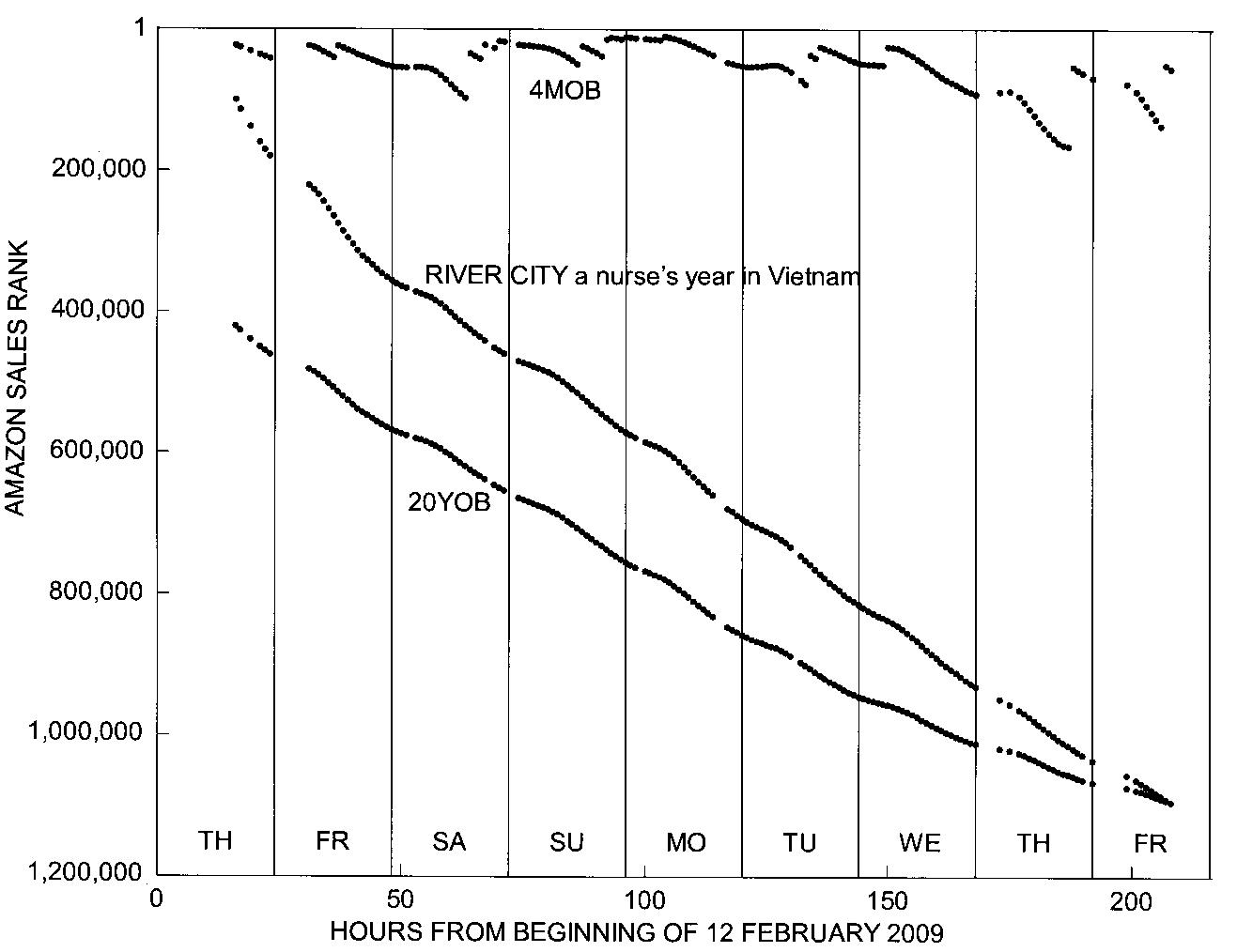
Figure 1.
Figure
2 shows the time zone distribution of the
Aaron
Shepard provides a convenient way to check Amazon sales ranks with salesrankexpress.com which allows
you to store the query information for two books. It was used in the initial phase of data
collection for this analysis. The day
after the first sale of RIVER CITY on Amazon it was decided to accumulate the
sales rank data hourly. Amazon sales
ranks generally update at about five or ten minutes before the hour. If you wake up at quarter to the hour you can
get the previous hour’s rank before the update, get the next hour’s rank after
the update, then go back to bed for an hour and forty-five minutes. After six days, exhaustion set in and the
quest for hourly data was abandoned.
In
May, rankforest.com was
discovered and acquisition of hourly sales rank data on RIVER CITY was resumed. For a $6/month membership fee rankforest.com will collect all 24
Amazon sales ranks each day for you to export.
The sales ranks are tagged year round in daylight savings time in the
The
overall sales rank question will be approached by addressing two component
questions. How does not selling a book
affect your Amazon sales rank? How does
selling a book affect your Amazon sales rank?
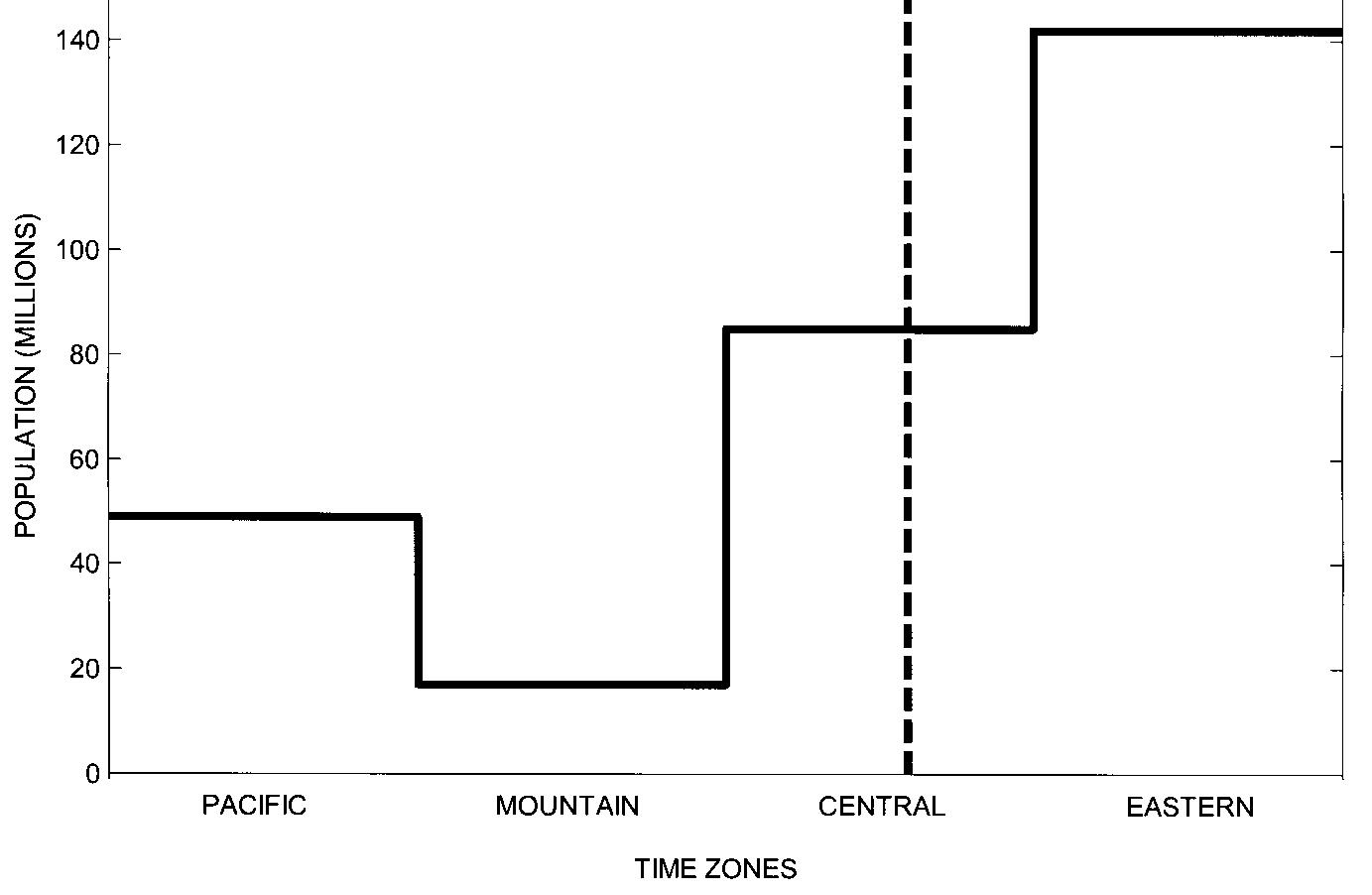
Figure 2.
How does not
selling a book affect your Amazon sales rank?
Neither
RIVER CITY nor 20YOB sold a book during
the eight day interval shown in Figure 1 and both their sales ranks increased
monotonically over that interval.
Although the sales rank of RIVER
CITY was about 300,000 lower that 20YOB initially, Amazon afforded the
newcomer less respect and its status decayed more rapidly, resulting in a
greater sales rank than 20YOB by the end of the eight days.
It
appears that Amazon assigns an average status decay rate to books based on both
their present sales rank and their long term history. Figure 3 shows a progression of decay curves
for RIVER CITY. The green curve is identical to the one in
Figure 1 after the first Amazon sale on 12 February. The blue curve shows a slower decay after the
second Amazon sale on 21 February, although it still reached almost 1,700,000
before the next sale. The red curve
shows the sales rank actually leveling off at about two weeks after a sale in
mid-October before continuing the status decline. There also seems to be an inflection point
two weeks after the sale on 21 February.
All three curves have about the same decay rate for sales ranks less
than 200,000.
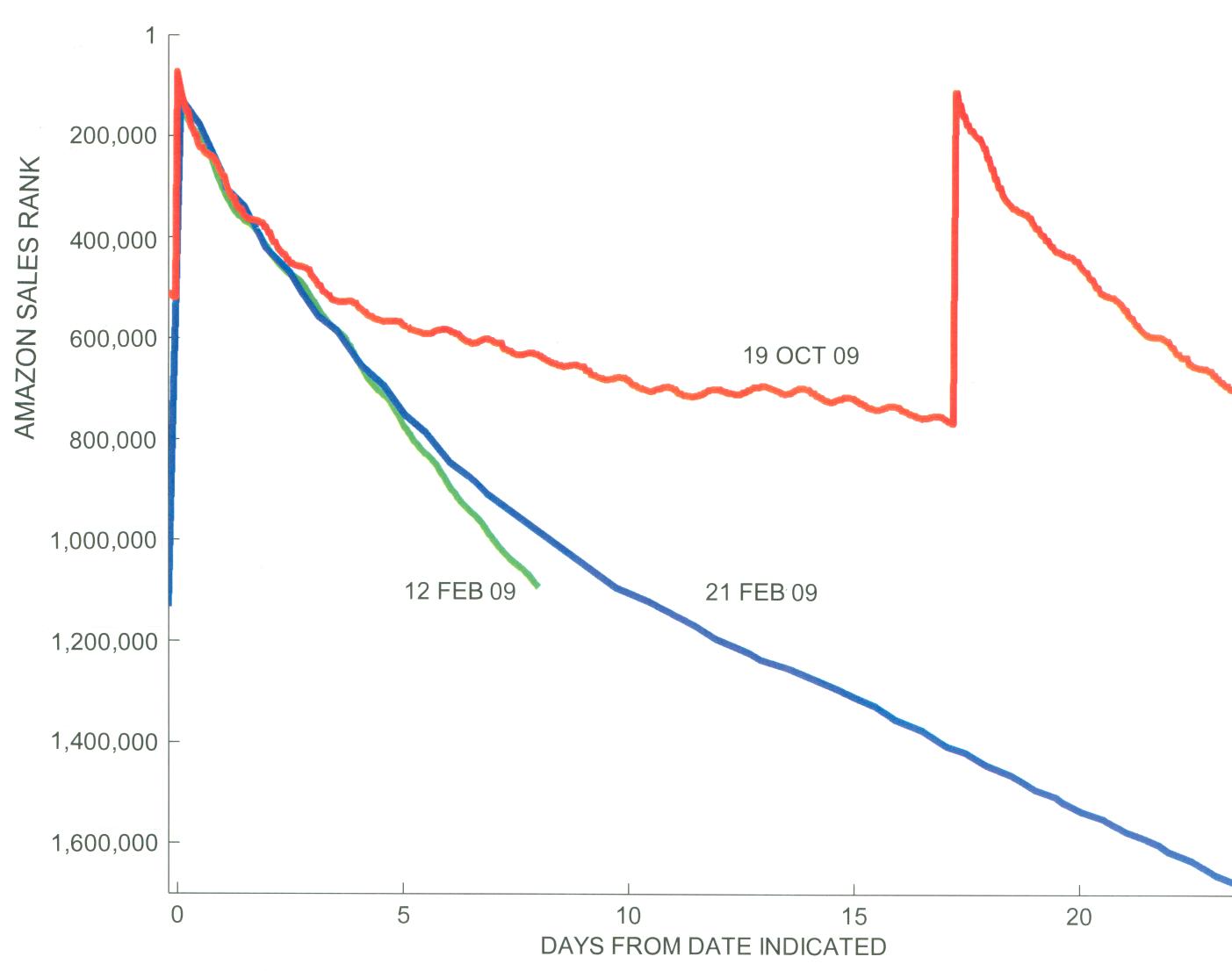
Figure 3.
Figure
4 shows data from three different days spanning more than a month during the
summer. The circles indicate the
variation of sales ranks over portions of each day when no copy of RIVER CITY sold on Amazon. Although Amazon nominally updates sales ranks
hourly, the values will frequently be identical for two or three hours in a
row. The curves in Figure 4 were generated
by applying a cubic spline interpolation to the sales ranks that were not
frozen. The three curves, which are
almost identical in shape, make it easy to visualize what the frozen sales rank
values should have been. The frozen
values occur randomly but when they do, the sales ranks for all books fail to
update. It is as if some glitch
interrupted the computation for a given hour but did not disturb the values at
later times.
The
most gentle slope for each curve in Figure 4 is around 5 a.m. and the steepest
slope is around noon. This diurnal
oscillation is also apparent in Figures 1 and 3. Figure 5 makes that characteristic in the
Figure 1 data more apparent by plotting the change in the sales rank for each
adjacent pair of points divided but the difference in the observation times. The result is the change in sales rank per
hour, plotted midway between the two observations. That allows consistent changes to be computed
even across large data gaps, although those points are certainly less accurate
than when the observations are an hour apart.
What
is apparent in Figure 5 is a pronounced diurnal oscillation about the mean
trend in sales rank when no sale occurs.
The magnitude of the oscillation is similar for all three books. The sales rank increases most rapidly in the early
afternoon and it increases most slowly around 5 a.m. That seems reasonable. If you haven’t sold a book, but it is 5 a.m.
and very few books are selling, you shouldn’t be penalized. But if you haven’t sold a book at noon when
lots of books are selling, you’re going to lose status fast.
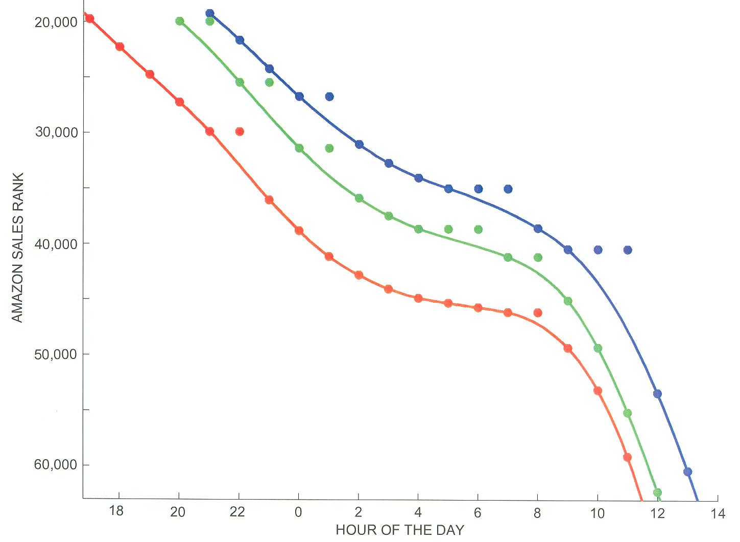
Figure 4.
It
is interesting that most of the diurnal variations are very similar. There is a peak in the early afternoon
followed by a sharp drop, then a sort of shoulder in the evening. The points for 4MOB are more scattered
because it was selling books during this period. That will be addressed in the next
section.
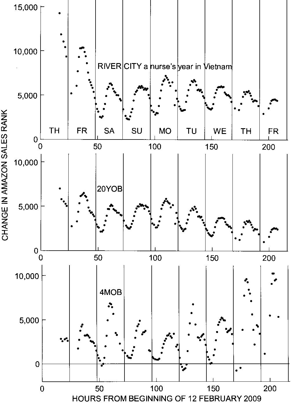
Figure 5.
One
might intuitively expect that the status of a book would decay in any hour in
which no sale occurred, which was true for both RIVER CITY and 20YOB in Figures 1 and
5. But the situation is more complex and
the sales rank of 4MOB actually decreased in Figure 5 for several hours after
hour 120, evidenced by the negative changes in sales rank, even though no sales
occurred.
The
algorithm Amazon uses to determine sales rank in the absence of a sale seems to
have two parts. There appears to be a
mean decay rate, based on sales history and present sales rank, and an
oscillation about the mean rate whose amplitude is probably based on the total
sales of all books during that hour. The
amplitude of the oscillation does not seem to be affected by the mean decay
rate. So if the mean decay rate is slow,
the oscillation can actually cause the sales rank to decrease without a sale in
the early morning hours. This happened
often in the case of the 19 October curve in Figure 3.
Figure
6 shows a scatter plot of all the changes in sales rank for two books during
hours when they sold no copy on Amazon.
The books were RIVER CITY and a
three month old book (3MOB) published in October 2009. The criteria for each sales rank change used
in the scatter plot was that the previous and following sales rank values had to
be different from the present value, and the three values had to be separated
by one hour. This simple procedure
ensured that no frozen values (Figure 4) contaminated the computation and that
the accuracy of the change in sales rank was not degraded by time gaps in the
data. A great deal of data were
eliminated by the criteria, but enough remained to provide a quantitative
picture of Amazon sales rank decay rates.
Most
of the data points in Figure 6 are for sales ranks less than 100,000. The circles indicate the average values of
all the changes in sales rank in 25,000 interval bins (0-25,000, 25,000-50,000,
50,000-75,000, …). Changes in sales rank
larger than 18,000 were considered outliers and excluded from the
averages.
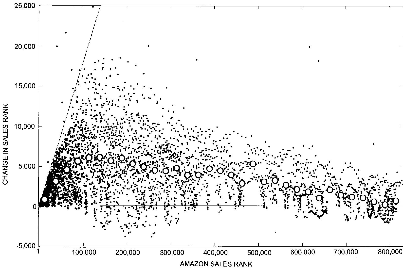
Figure 6.
The
diurnal oscillation in sales rank decay rates spreads out the sales rank
changes vertically, sometimes causing them to go negative and actually decrease
the sales rank, but the circles provide a good overall view of the average
sales rank decay rate as a function of sales rank. Sales rank status decays most rapidly for
sales ranks in the 100,000-150,000 range.
For higher sales ranks the decay rate decreases approximately linearly
with increasing sales rank to a small value at about 800,000.
An
interesting feature is indicated by the dashed line in Figure 6 which has a
slope of 0.18 and, for the most part, provides an upper limit on the changes in
sales rank. What it indicates is that if
you have a high status (low sales rank), that status will decay slowly if you
don’t sell a book in a given hour. But
as your status does decay, the decay rate will accelerate, shoving you down
faster and faster until your sales rank exceeds 150,000. Once your status is that low, Amazon starts
easing up on you and your status diminishes at a slower and slower rate.
Figure
7 shows idealized Amazon sales rank decay rate plots generated for use in a
simulation. The first six circles are
identical to the ones in Figure 6. The
circles for sales ranks larger than 150,000 are a linear approximation of the
mean trend in Figure 6, with the change in sales rank arbitrarily fixed for
sales ranks greater than 800,000. Amazon
might apply fixed sales rank decay rates for sales ranks below 150,000 (first
six circles in Figure 7) and then vary the decay rates for larger sales ranks
depending on your recent and cumulative sales (dashed lines in Figure 7). The steep dashed curve would slow your status
decline and the shallow dashed curve would move you more rapidly toward higher
sales ranks.
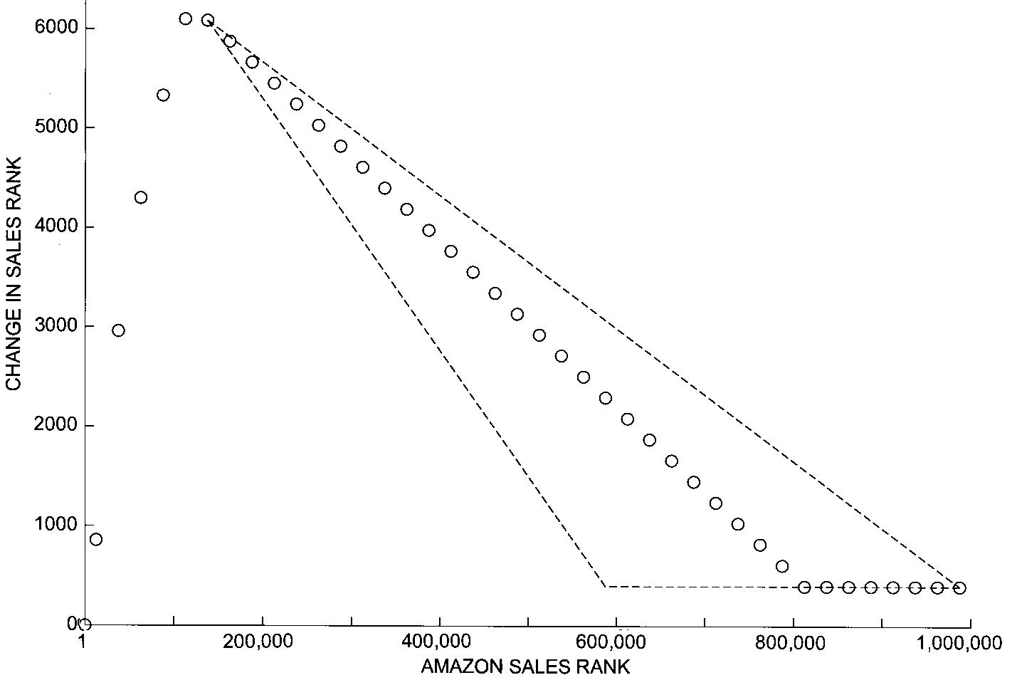
Figure 7.
The
distribution of sales rank increases shown in Figure 7 helps better selling
books maintain their status. The lower
your sales rank, the slower the initial increase in sales rank if you go
several hours without a sale. Figure 8 shows
the effect the three curves in Figure 7 would have on two books which achieved
sales ranks of 1,000 (red) and 3,000 (blue) and then stopped selling. The thick curves are actually composed of a
sequence of dots indicating the hourly sales rank variation over the three week
period corresponding to the circles in Figure 7. The upper and lower dashed curves in Figure 8
correspond to the lower and upper dashed curves in Figure 7.
The
Amazon respect for status is relatively short lived. What appears to be a plateau during the first
day (blue) or two (red) in Figure 8 is actually a significant decay in status
apparent in the enlargement shown in Figure 9.
For the book with an initial sales rank of 3,000, the sales rank triples
in about 19 hours and has increased by a factor of 10 after a day and a half
without a sale. The sales rank for the
book starting at 1,000 triples in just over 20 hours. After that it follows the same sales rank
increase trajectory as the blue book, but with a 20-hour lag.
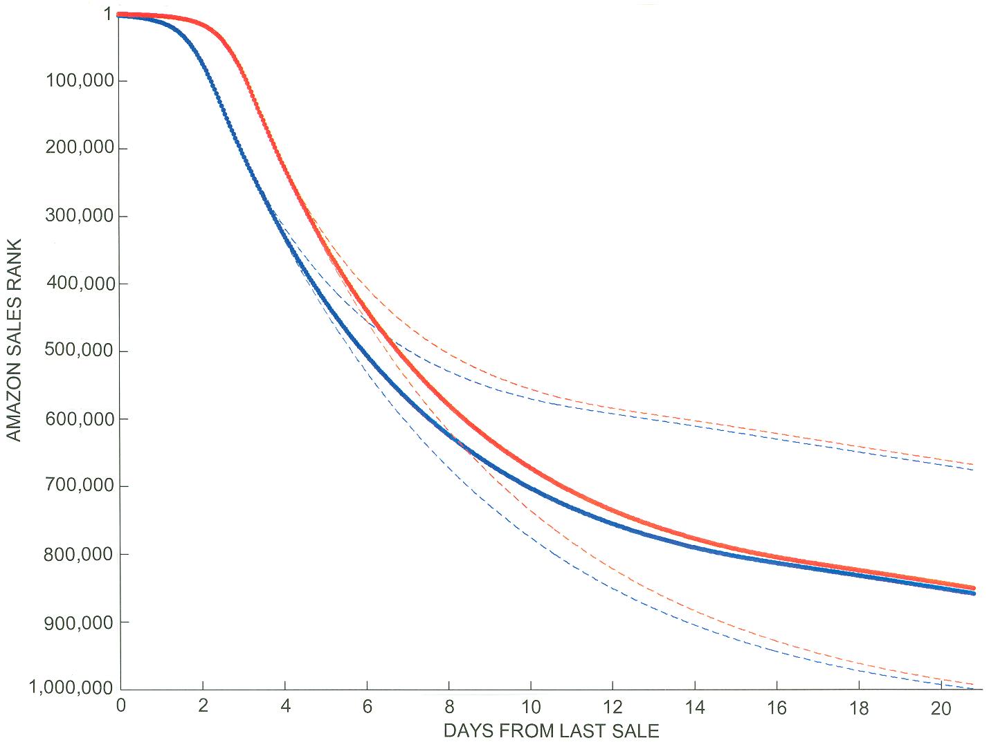
Figure 8.
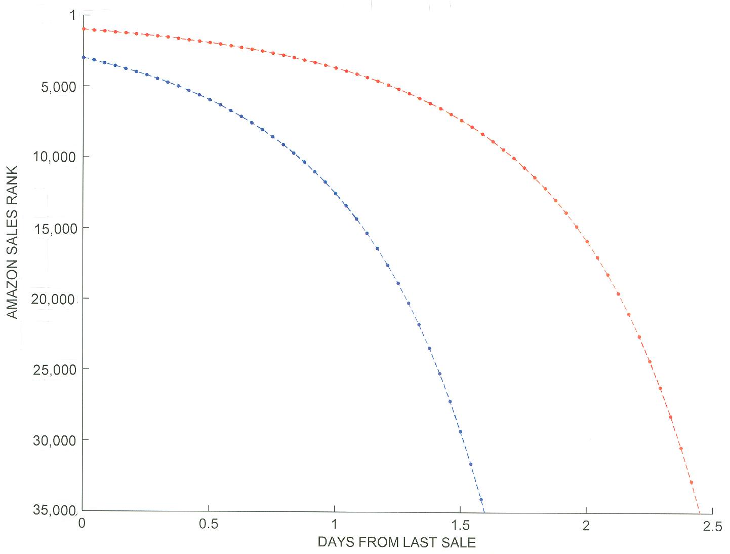
Figure 9.
The
diurnal oscillation was not factored into the sales rank decays shown in
Figures 8 and 9 but will be incorporated in the overall sales rank simulation
developed in the next section. Figure 10
shows the diurnal variation used, which seemed to well approximate the
variation for sales ranks less than 100,000.
To obtain the sales rank decay for any given hour without a sale, the
mean decay rate (Figure 7) corresponding to the sales rank of the previous hour
would be multiplied by the diurnal oscillation factor (Figure 10) corresponding
to the present hour of the day. The
resulting increase in sales rank would vary by almost an order of magnitude
depending on the time of day. Another
important aspect of Figure 10 is that one might be able to monitor the sales
rank decay rate and use it as a surrogate for how total book sales on Amazon
varied throughout any given day. Such an
investigation would probably show significant differences between the weekday
and the weekend distributions.
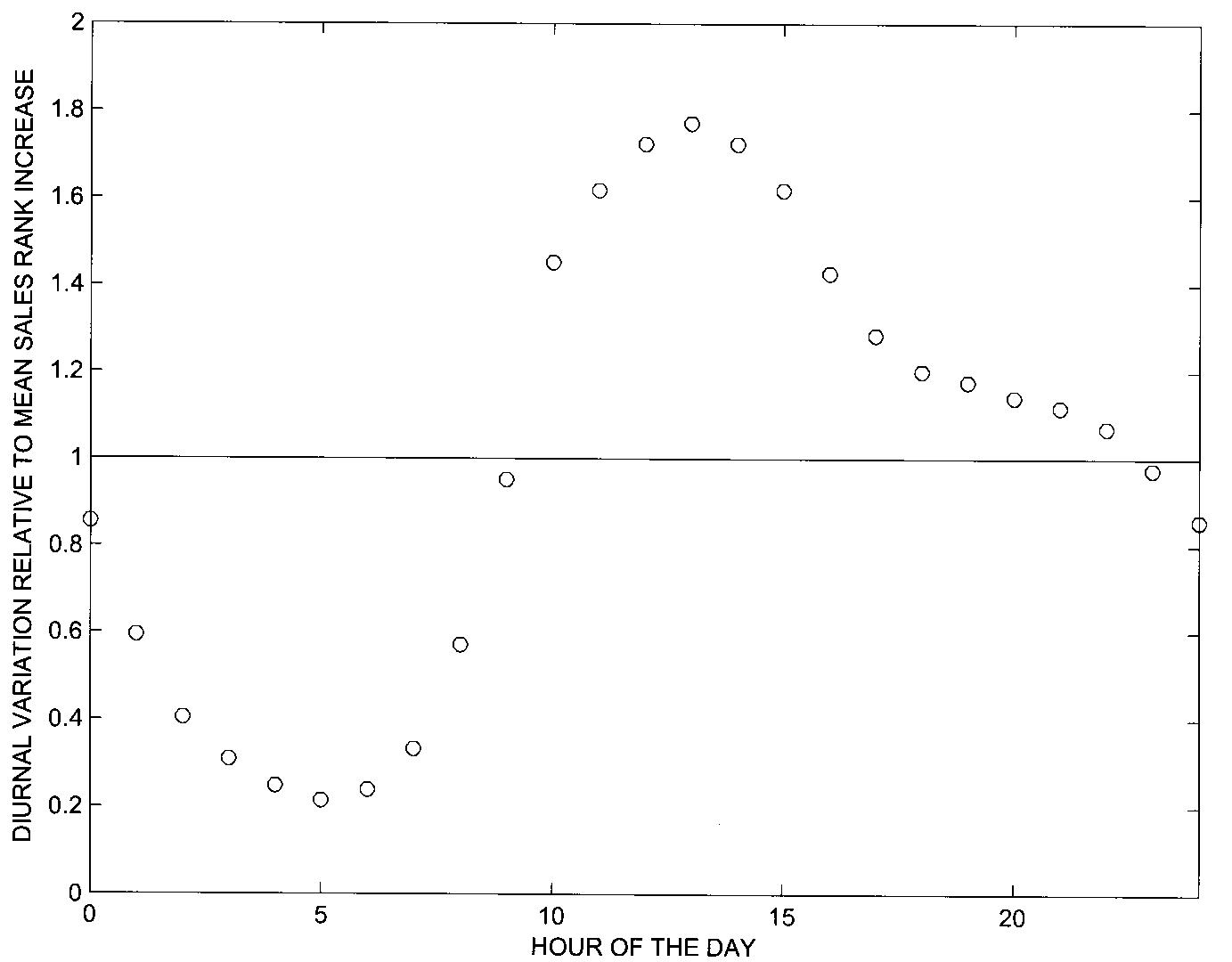
Figure 10.
How does
selling a book affect your Amazon sales rank?
Morris Rosenthal has provided an excellent
analysis of the significance of Amazon sales rank and its relationship to the
average number of books sold. His data
will be used to put the present analysis in perspective. It would be possible for Amazon to make a
straight forward sales rank calculation for the top several hundred books. The book that sold the most copies in the
previous hour would be number 1. The
book that sold the second most copies would be number 2, and so on. But that procedure would already break down
by sales rank 900. Rosenthal indicates
that books with sales ranks between 800 and 1,000 are selling about 30 books
per day. With 200 books each selling
about one or two an hour, Amazon could not order them into unique sales ranks
on that basis. Even considering the
total number of books sold in the previous 24 hours and updating that number
each hour would not be able to differentiate between the books.
For
Amazon sales ranks between 3,000 and 140,000, Figure 11 indicates the number of
books sold per day, extracted from Morris Rosenthal’s graphs at http://www.fonerbooks.com/surfing.htm. With the sale of its first book on Amazon, RIVER CITY jumped past millions of other
books to a sales rank of 100,044. That
status was not actually unreasonable since the first sale guaranteed that RIVER CITY was selling at least one book
per day. When no book sold in the next
hour its status began a rapid decay.
Figure 11 indicates that a book selling one copy a day would have a sales
rank of about 140,000. It was not
possible to determine the average RIVER
CITY sales rank over the first 24-hour interval because of the missing
data, but it was probably about 200,000.
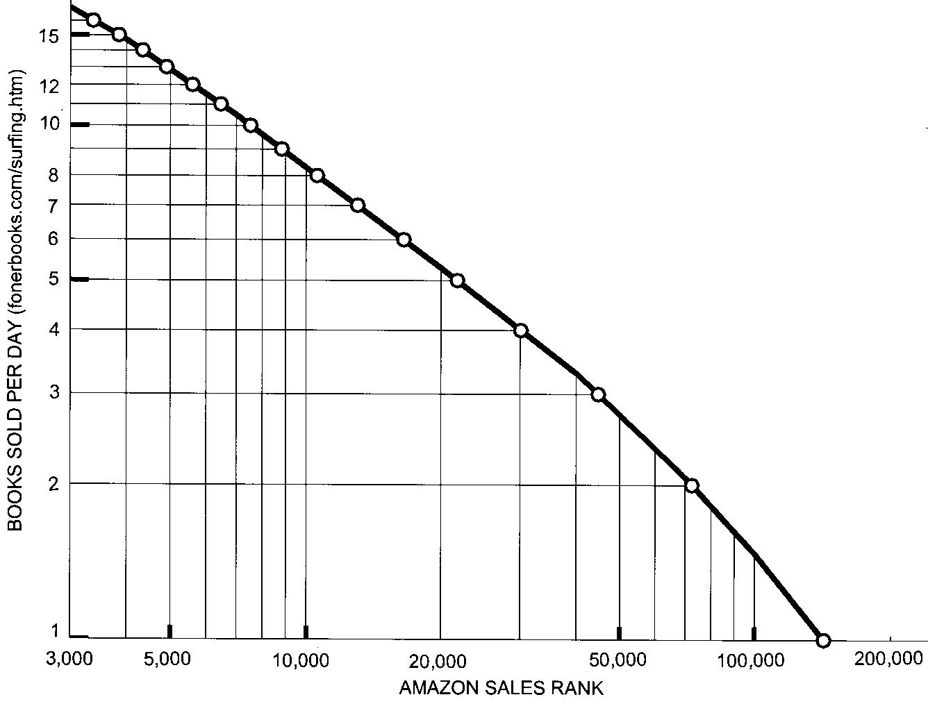
Figure 11.
The
sales rank variation of 4MOB in Figure 1 exhibits what some refer to as erratic
behavior, but the blowup shown in Figure 12 indicates the kind of information
that can be gleaned. Vertical lines have
been drawn in Figure 12 to indicate the fifteen times during the eight day
period that contained sales of 4MOB. On
one of the days (Sunday, hours 72 to 96), sales were made during four different
hours (with the final sale just before midnight). One day had sales in each of three different
hours, two days had sales in each of two hours, and four days had sales only
during one hour.
With
so few hours when books were sold, it is not unreasonable to assume that only
one book sold during any particular hour.
An interesting insight from this assumption is that the larger the sales
rank, the larger the decrease in it from the sale of a book. The lower the starting position in Figure 12,
the greater the vertical jump. As a
reminder, the circle at 100,044 near the left edge indicates the jump from
infinity that RIVER CITY made with the
sale of its first book on Amazon. For
sales ranks less than 20,000, the decrease with the sale of a single book is
relatively small. Of course, the jump at
about hour 30 in Figure 12 is an estimate assuming that the sales rank just
decayed over the missing data interval.
The
important point is that once one recognizes that the diurnal oscillations in
the no-sale decay rate can slightly reduce sales rank without a sale (during
the early morning hours of Tuesday and Thursday in Figure 12, for example), the
actual hours when sales occur become quite obvious. The same general characteristics are on
display in Figure 13 for the sales rank variation of 3MOB published in October
2009. Because the average sales of 3MOB
during the interval shown in Figure 13 were higher than those of 4MOB in
February 2009, it can be used to provide additional insights.
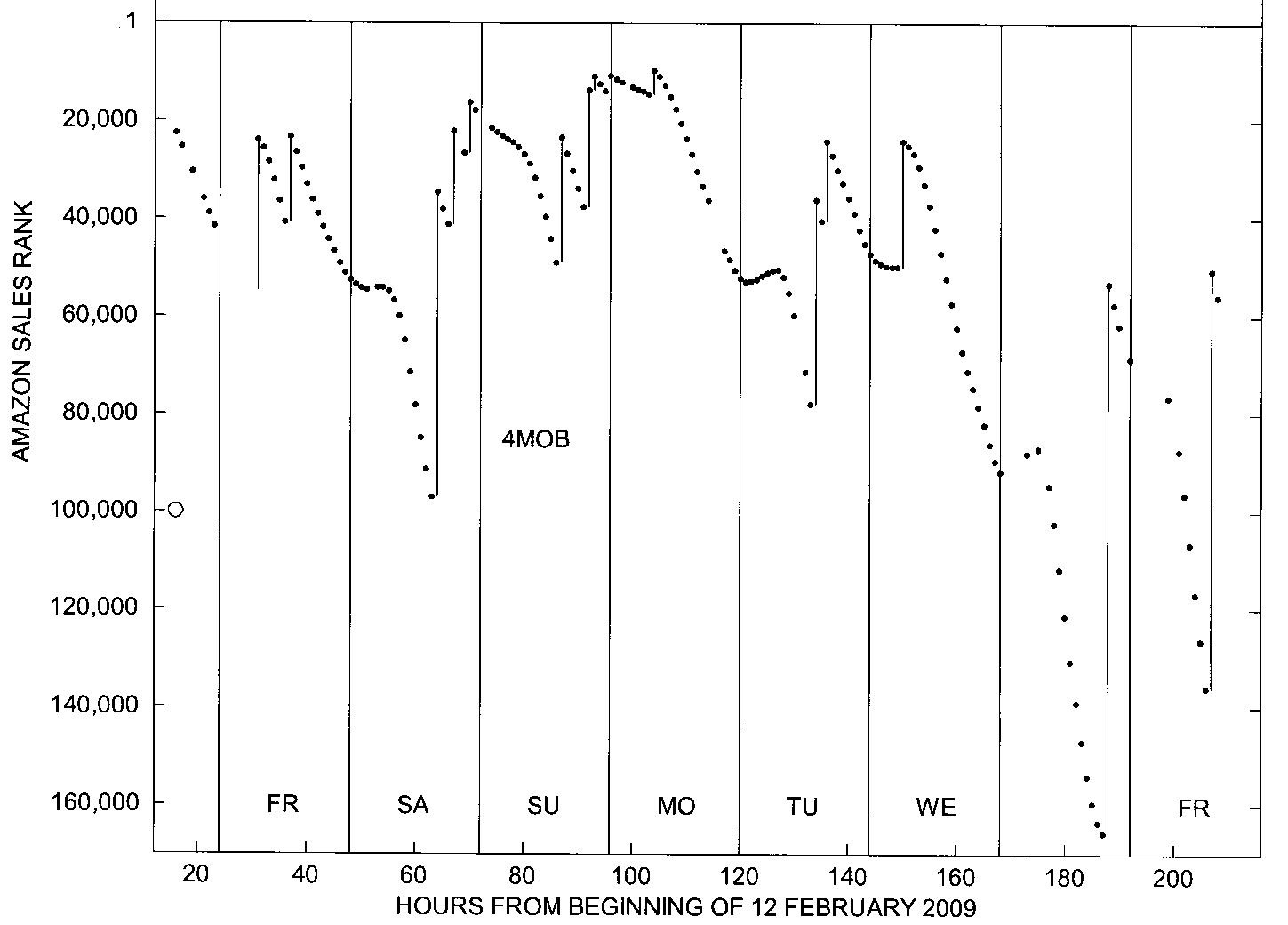
Figure 12.
The
top panel of Figure 13 shows the sales rank variation of 3MOB during the first
23 days of December. Figure 4 showed
typical occurrences of frozen sales ranks, but during the first three days of
December there were both 18-hour and 11-hour intervals when the Amazon sales
ranks did not update. During the first
three days there were also three 3-hour intervals and five 2-hours intervals
when the sales ranks did not update.
Sales ranks frozen for long intervals are uncommon, but sales ranks not
updating for a two or three hour interval once or twice a day are not
unusual.
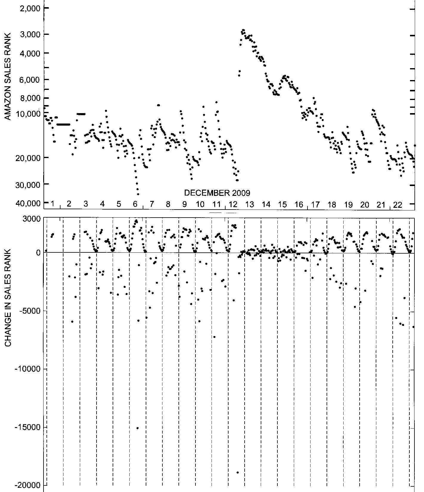
Figure 13.
Since
the sales rank data acquired for 3MOB (and RIVER
CITY after late May) were hourly without gaps, thanks to rankforest.com, the same strict
editing criteria used for Figure 6 were applied in quantifying changes in sales
rank resulting from a sale. The previous
and following sales rank values had to be different from the present value, and
the three values had to be separated by one hour. So no frozen values (Figure 4) contaminated
the computations and the accuracy of the change in sales rank was not degraded
by time gaps in the data.
The
bottom panel of Figure 13 shows all the changes in sales rank, both positive
and negative, that satisfied the editing criteria. The dashed lines in Figure 13 are located at
5 AM each day. The diurnal oscillation
in sales rank decay during hours without a sale is readily apparent during two
intervals, December 3-12 and 16-23.
There appears to have been a promotional push on December 12 that pumped
up sales of 3MOB for a few days. Figure
11 indicates that a sales rank of 3,000 corresponds to selling about 17 books
per day, averaging more than one per hour during the late morning - early
afternoon peak selling interval (Figure 10), suppressing the diurnal
oscillation in sales rank decay.
Figure
11 indicates that books with sales ranks of 10,000 or larger are selling about
8 copies a day or less. That seems like
a reasonable threshold for assuming that only one book will sell in any given hour. By looking at the negative excursions in
sales rank in the bottom panel of Figure 13 when the sales rank is 10,000 or
larger in the top panel, you can get the same general impression of the effect
of a sale as was apparent in Figure 12.
The lower the starting position (higher sales rank) in the top panel,
the greater the jump. While the sales
rank is small during December 13-15 the reductions in sales rank are quite
modest, even if more than one book sold in an hour, as might have occurred.
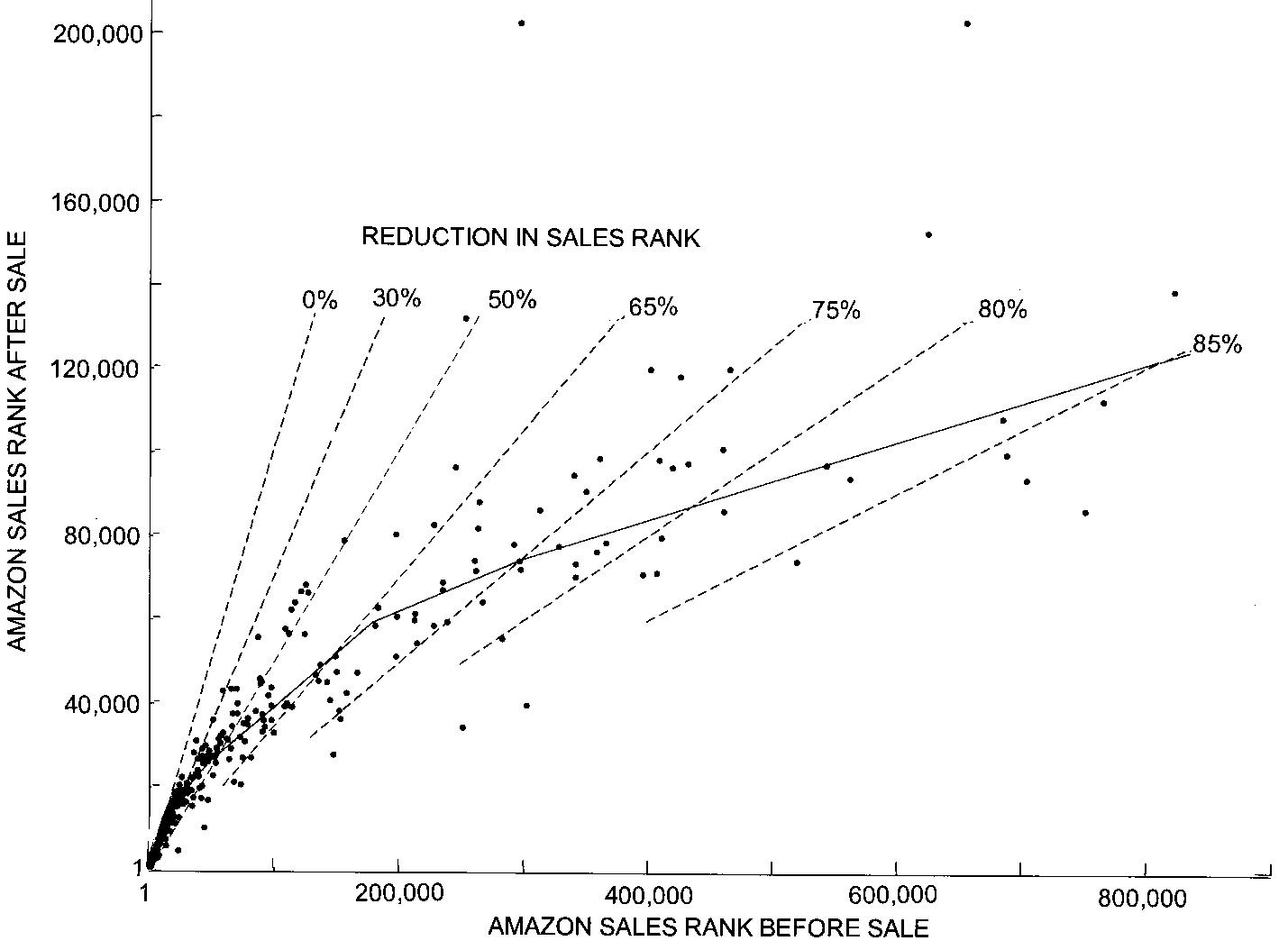
Figure 14.
The
dots in Figure 14 show the relationship between the sales ranks of 3MOB and RIVER CITY before and after each hour in
which a sale occurred. The dashed curves
show the positions within the scatter plot for which the sales of a single book
would cause the sales rank to be reduced by 85%, or 80%, or 75%, … When the sales rank is about 750,000, the
sale of a single book will generally bring it down to around 100,000, a
reduction of about 85%. When the starting
sales rank is lower, the percent reduction is also lower.
There
is a significant amount of scatter in Figure 14, which is reasonable
considering the time interval covered is May 2009 through January 2010 for RIVER CITY and October 2009 through
January 2010 for 3MOB. Morris Rosenthal
indicates that the data of Figure 11 represent an average behavior and that
there are weekly to seasonal variations in sales as well as trends over longer
time periods. The solid curve in Figure
14 was used as a piecewise linear approximation of the average variation of the
change in sales rank resulting from the sale of a single book.
Figure
15 shows an enlargement of Figure 14 for sales ranks less than 100,000. The minimum reduction in sales rank for the
piecewise linear approximation (solid curve) is fixed at 10.7% for sales ranks
of 15,000 or less. As was indicated
earlier, the reductions in sales rank used in this analysis were assumed to
have resulted from the sale of a single book.
That assumption would tend to break down for sales ranks lower than
10,000. The % reduction in sales rank
per copy sold for books in low sales ranks which sell many an hour would have
to be much less than 10.7%. For example,
Morris Rosenthal indicates books with sales ranks of about 900 sell roughly 30
a day on average. Amazon would probably
increase the sales rank for such a book if it only sold one copy in an hour
during the middle of the day. The solid
curve in Figure 15 indicates that the sales rank would decrease by 96. So this analysis would not be valid for books
with sales ranks much less than 10,000.
But sales ranks of 10,000 and greater encompass 99.8% of all the books
for sale at Amazon.com.
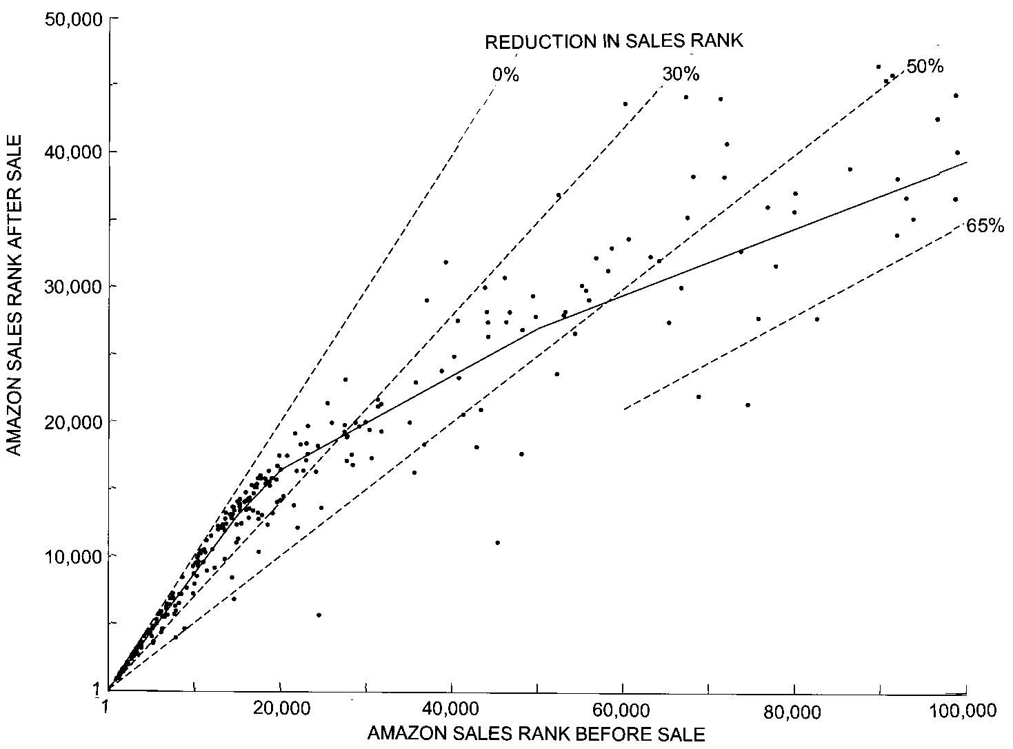
Figure 15.
The
final step taken to assess the reasonableness of this analysis was to run an
overall simulation of the variation of sales rank assuming that a book started
selling 1, 3, 5, or 7 copies a day on Amazon.
Figure 16 shows the sales rank variation over a two week period for a
book with an initial sales rank of 800,000 that started selling one book a
day. The blue dots indicate the hourly
sales rank values if the book sales always occurred at 5 AM. The red dots indicate the hourly sales rank
values if the book sales always occurred at 1 PM.
If
no sale occurred in a given hour, the average sales rank decay rate (circles in
Figure 7) corresponding to the sales rank of the previous hour was multiplied
by the diurnal coefficient for that hour of the day (Figure 10) to get the
actual increase in sales rank. For each
hour in which a sale occurred, the new reduced sales rank was determined from
the piecewise linear approximation (solid curve) of the average reduction in
sales rank indicated in the scatter plot shown in Figures 14 and 15.
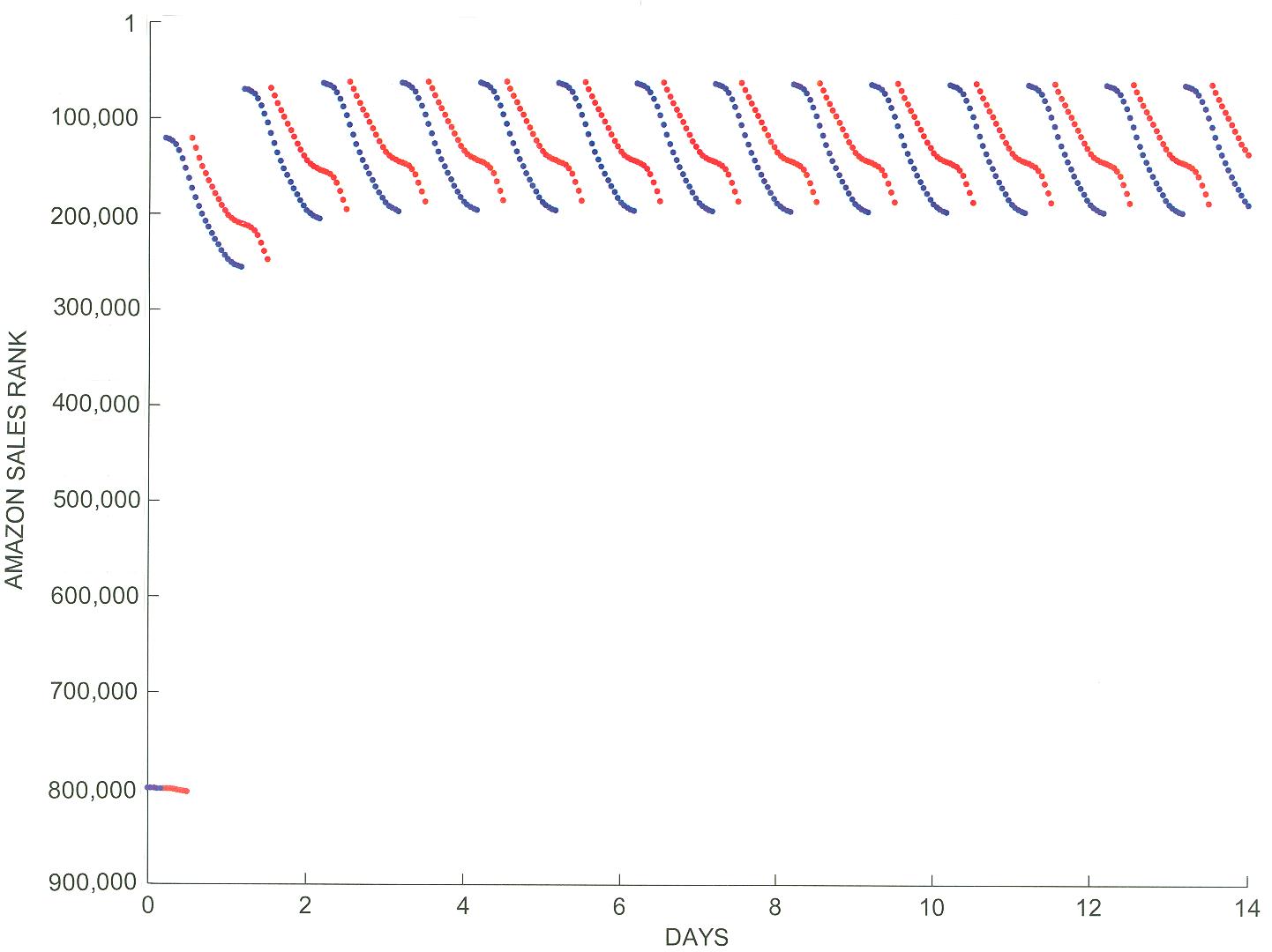
Figure 16.
The
daily variation in sales rank shown in Figure 16 stabilized after about four
days and there was not much difference in the mean values of the red and blue
distributions. The bottom panel of
Figure 17 shows an enlarged portion of Figure 16 to compare with similar
enlargements for sales of 3, 5, or 7 books per day shown in the upper
panels. The multiple sales in a day were
assumed to occur one in each sequential hour centered on either 5 AM (blue) or
1 PM (red). The initial sale in all
cases reduced the sales rank to about 120,000.
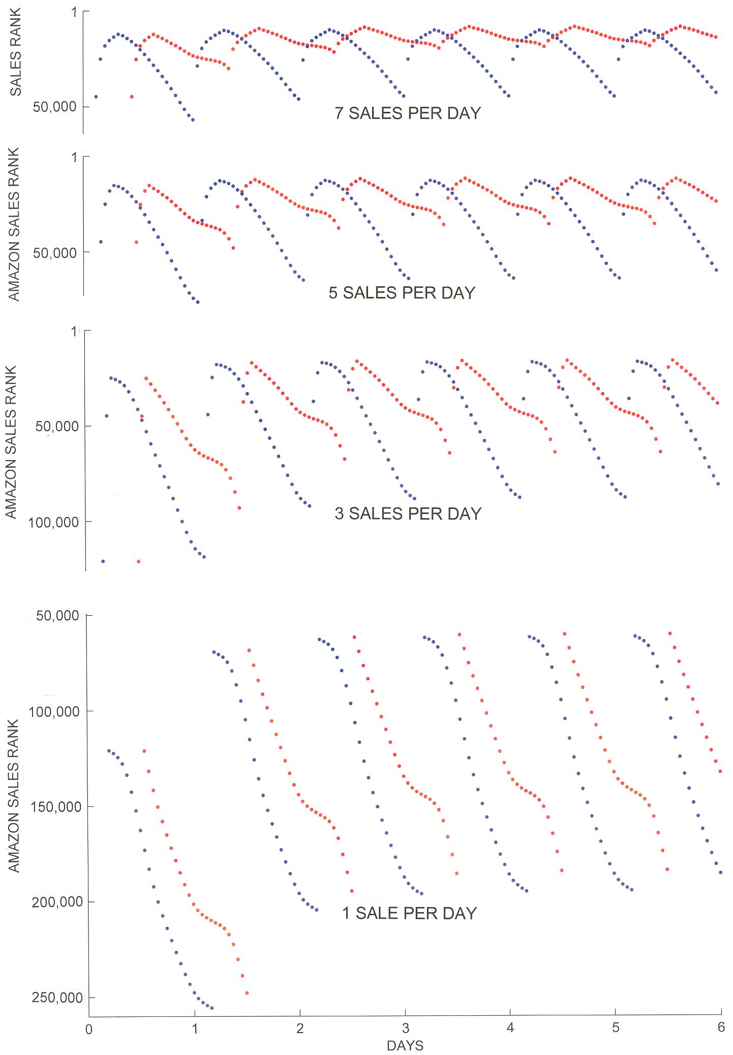
Figure 17.
When
there is only one sale per day, the sales rank immediately begins to
increase. When there are multiple sales
in a day, the sales rank continues to decrease during the interval of sales,
but by a smaller amount each time the sales rank is reduced (Figures 14 and
15). Once the sales conclude for the day
the sales rank increases hourly until sales resume the following day. In this algorithm the time of day when a sale
occurs is important. In the top panel of
Figure 17 the seven reductions in sales rank which were centered on 1 PM (red
dots) took the place of the seven largest increases in sales rank that would
have occurred had there been no sale (Figure 10). In contrast, the blue dots showing the seven
reductions in sales rank which were centered on 5 AM replaced the seven
smallest increases in sales rank that would have occurred had there been no
sale. With no sales in the late morning
and early afternoon, the sales rank of the blue dots increased relatively
quickly because of the diurnal variation (Figure 10), resulting in an average
sales rank for the blue dots that is significantly larger than the average
sales rank of the red dots, even though the same number of books were sold.
Figure
18 repeats the Morris Rosenthal curve from Figure 11 to which the average sales
ranks resulting from the simulation (Figure 17) have been added. The red dots for the sales centered on 1 PM
are remarkably close to the Rosenthal curve while the blue dots for the sales
centered on 5 AM tend to have significantly larger sales ranks for the same
number of books sold. It is reasonable
that the red dots should be closer to the curve since midday is the most likely
time for people to buy books and that is why the diurnal variation curve
(Figure 10) has the shape it does.
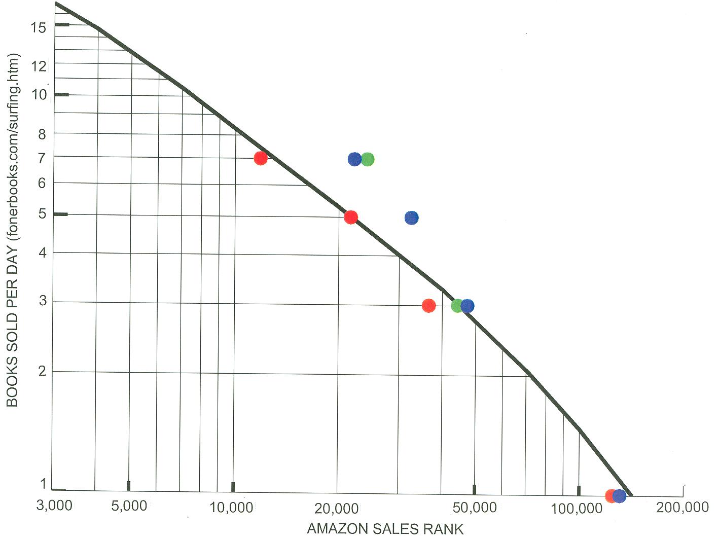
Figure 18.
Although
the algorithm developed here was based on statistics assuming that only one
book sold in any given hour, it can be applied to books selling multiple copies
an hour as long as the sales rank of the book is not too low. If a book happened to sell five copies in an
hour, you would sequence through the sales rank reduction process five times in
a row, just as you would if the sales occurred in sequential hours. The difference is that if all the sales
occurred in a single hour, the sales rank will immediately begin to grow in
subsequent hours and you will end up with a higher sales rank than if the sales
had been spread out over time. There are
three green circles on Figure 18, although only two of them are visible. They correspond to books which sold 3, 5, or
7 copies a day, but with all sales occurring exactly at 1 PM. For the book selling 3 copies a day at 1 PM,
the sales rank is only a little lower than the book whose sales were spread out
around 5 AM. For the book selling 5
copies a day at 1 PM, the green circle is directly behind the blue circle. For the book selling 7 copies a day at 1 PM,
the sales rank is higher than the book which sold its 7 copies spread out
around 5 AM. Your sales rank will be
lowest if your books sell midday and spread out over time.
As
a general conclusion of this analysis, it seems likely that, for books whose
sales ranks are about 10,000 or greater, Amazon uses a mathematical algorithm
to determine the sales rank of each book that does not depend on what is
happening to the sales rank of any other book in that range. One might naively think that in every hour
Amazon places several million books into a unique sales rank order, but that is
probably not the case. In any given
hour, who would know if two books had the sales rank 253,761 and no book had
the sales rank 253,760? If any book with
a sales rank greater than 10,000 doesn’t sell during a given hour, Amazon seems
to just increase its sales rank by the amount indicated for its present sales
rank and sales history (Figure 7), modified by a function of the total sales
during that hour (Figure 10). If a book
does sell, they seem to just decrease its sales rank by some amount that is
determined by its present sales rank (Figures 14 and 15).
If
Amazon were doing something more complex, the diurnal variation seen in Figure
10 probably would not exist in the changes they make to sales ranks. In fact, if a book sold 7 copies a day, day
after day, it really should have the same sales rank whether those copies all
sold in one hour, or the sales were spread out over a number of hours in any
part of the day. But then Amazon would
have to consider an entire day’s sales and could not update sales rank on an
hourly basis. Amazon may well monitor
how many books are in various sales rank ranges (50,000-100,000,
100,000-150,000, 150,000-200,000, …) to see if the coefficients they are using
are producing reasonable results statistically.
If there are about 50,000 books in each bin, the various coefficients
would be doing a decent job of showing authors what their status is. If books were starting to bunch up in certain
bins, the coefficients would need adjustment.
[home page] [How does Amazon determine sales rank?] [Contact Information] [Biographical Notes]
These pages are copyright ©1998-2013 by Patricia L. Walsh